2  Data visualization

2.1 Notes

alpha aesthetic to add transparency to the filled density curves.

This aesthetic takes values between 0 (completely transparent) and 1 (completely opaque)

is to split your plot into facets, subplots that each display one subset of the data.

To facet your plot by a single variable, use facet_wrap(). The first argument of facet_wrap() is a formula2, which you create with ~ followed by a variable name. The variable that you pass to facet_wrap() should be categorical.

2.2 Questions

Make a scatterplot of hwy vs. displ using the mpg data frame. Next, map a third, numerical variable to color, then size, then both color and size, then shape. How do these aesthetics behave differently for categorical vs. numerical variables?

that second part of the question is really unclear to me

3.In the scatterplot of hwy vs. displ, what happens if you map a third variable to linewidth?

i don’t know how to map a third variable??

2.3 2.2.5 Exercises

1.How many rows are in penguins? How many columns?

344 rows and 8 columns

library(tidyverse)
── Attaching packages ─────────────────────────────────────── tidyverse 1.3.2 ──
✔ ggplot2 3.4.0     ✔ purrr   1.0.1
✔ tibble  3.1.8     ✔ dplyr   1.1.0
✔ tidyr   1.3.0     ✔ stringr 1.5.0
✔ readr   2.1.3     ✔ forcats 1.0.0
── Conflicts ────────────────────────────────────────── tidyverse_conflicts() ──
✖ dplyr::filter() masks stats::filter()
✖ dplyr::lag()    masks stats::lag()
library(palmerpenguins)


glimpse(penguins)
Rows: 344
Columns: 8
$ species           <fct> Adelie, Adelie, Adelie, Adelie, Adelie, Adelie, Adel…
$ island            <fct> Torgersen, Torgersen, Torgersen, Torgersen, Torgerse…
$ bill_length_mm    <dbl> 39.1, 39.5, 40.3, NA, 36.7, 39.3, 38.9, 39.2, 34.1, …
$ bill_depth_mm     <dbl> 18.7, 17.4, 18.0, NA, 19.3, 20.6, 17.8, 19.6, 18.1, …
$ flipper_length_mm <int> 181, 186, 195, NA, 193, 190, 181, 195, 193, 190, 186…
$ body_mass_g       <int> 3750, 3800, 3250, NA, 3450, 3650, 3625, 4675, 3475, …
$ sex               <fct> male, female, female, NA, female, male, female, male…
$ year              <int> 2007, 2007, 2007, 2007, 2007, 2007, 2007, 2007, 2007…

2.What does the bill_depth_mm variable in the penguins data frame describe? Read the help for ?penguins to find out.

?penguins

a number denoting bill depth (millimeters)

3.Make a scatterplot of bill_depth_mm vs. bill_length_mm. Describe the relationship between these two variables.

ggplot(data = penguins, aes(x = bill_depth_mm, y = bill_length_mm)) + geom_point()
Warning: Removed 2 rows containing missing values (`geom_point()`).

#it looks like to me that there can be long narrow beaks and long wide beaks aswell as  shorter beaks that have more depth seems pretty balanced

4.What happens if you make a scatterplot of species vs bill_depth_mm? Why is the plot not useful?

ggplot(data = penguins, aes(x = species, y = bill_depth_mm)) + geom_point()
Warning: Removed 2 rows containing missing values (`geom_point()`).

5.Why does the following give an error and how would you fix it?

that code has no x or y mapping

6.What does the na.rm argument do in geom_point()? What is the default value of the argument? Create a scatterplot where you successfully use this argument set to TRUE.

the na.rm argument takes away the warning message. The default is false.

ggplot(data = penguins, aes(x = bill_depth_mm, y = bill_length_mm)) + geom_point(na.rm = TRUE)

7.Add the following caption to the plot you made in the previous exercise: “Data come from the palmerpenguins package.” Hint: Take a look at the documentation for labs().

ggplot(data = penguins, aes(x = bill_depth_mm, y = bill_length_mm)) + geom_point(na.rm = TRUE) + labs(caption = "Data come from the palmerpenguins package")

8.Recreate the following visualization. What aesthetic should bill_depth_mm be mapped to? And should it be mapped at the global level or at the geom level?

just at the geom level

ggplot(data = penguins,aes( x = flipper_length_mm, y = body_mass_g, color = bill_depth_mm)) + geom_point() + geom_smooth()
`geom_smooth()` using method = 'loess' and formula = 'y ~ x'
Warning: Removed 2 rows containing non-finite values (`stat_smooth()`).
Warning: The following aesthetics were dropped during statistical transformation: colour
ℹ This can happen when ggplot fails to infer the correct grouping structure in
  the data.
ℹ Did you forget to specify a `group` aesthetic or to convert a numerical
  variable into a factor?
Warning: Removed 2 rows containing missing values (`geom_point()`).

9.Run this code in your head and predict what the output will look like. Then, run the code in R and check your predictions.

it came out somewhat of what i thought it looked like i didn’t really understand the se = FALSE argument

ggplot(
  data = penguins,
  mapping = aes(x = flipper_length_mm, y = body_mass_g, color = island)
) +
  geom_point() +
  geom_smooth(se = FALSE)
`geom_smooth()` using method = 'loess' and formula = 'y ~ x'
Warning: Removed 2 rows containing non-finite values (`stat_smooth()`).
Warning: Removed 2 rows containing missing values (`geom_point()`).

10.Will these two graphs look different? Why/why not?

ya i think they will look the same because they are doing the same thing one is just writen out

ggplot(
  data = penguins,
  mapping = aes(x = flipper_length_mm, y = body_mass_g)
) +
  geom_point() +
  geom_smooth()
`geom_smooth()` using method = 'loess' and formula = 'y ~ x'
Warning: Removed 2 rows containing non-finite values (`stat_smooth()`).
Warning: Removed 2 rows containing missing values (`geom_point()`).

ggplot() +
  geom_point(
    data = penguins,
    mapping = aes(x = flipper_length_mm, y = body_mass_g)
  ) +
  geom_smooth(
    data = penguins,
    mapping = aes(x = flipper_length_mm, y = body_mass_g)
  )
`geom_smooth()` using method = 'loess' and formula = 'y ~ x'
Warning: Removed 2 rows containing non-finite values (`stat_smooth()`).
Warning: Removed 2 rows containing missing values (`geom_point()`).

2.4 2.4.3 Exercises

1.Make a bar plot of species of penguins, where you assign species to the y aesthetic. How is this plot different?

all it does is make the bars horizontal instead of vertical

ggplot(penguins, aes(y = species)) + geom_bar()

2.How are the following two plots different? Which aesthetic, color or fill, is more useful for changing the color of bars?

the first code outlines the bars while the second code completely shades in the bars,the second is more useful

ggplot(penguins, aes(x = species)) +
  geom_bar(color = "red")

ggplot(penguins, aes(x = species)) +
  geom_bar(fill = "red")

3.What does the bins argument in geom_histogram() do?

it determines the width or size of the bars

4.Make a histogram of the carat variable in the diamonds dataset. Experiment with different binwidths. What binwidth reveals the most interesting patterns?

glimpse(diamonds)
Rows: 53,940
Columns: 10
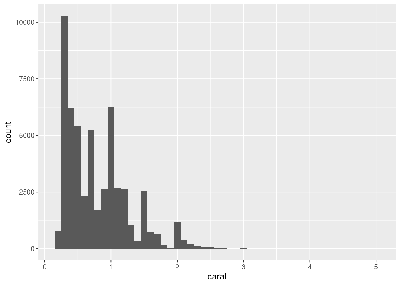
$ carat   <dbl> 0.23, 0.21, 0.23, 0.29, 0.31, 0.24, 0.24, 0.26, 0.22, 0.23, 0.…
$ cut     <ord> Ideal, Premium, Good, Premium, Good, Very Good, Very Good, Ver…
$ color   <ord> E, E, E, I, J, J, I, H, E, H, J, J, F, J, E, E, I, J, J, J, I,…
$ clarity <ord> SI2, SI1, VS1, VS2, SI2, VVS2, VVS1, SI1, VS2, VS1, SI1, VS1, …
$ depth   <dbl> 61.5, 59.8, 56.9, 62.4, 63.3, 62.8, 62.3, 61.9, 65.1, 59.4, 64…
$ table   <dbl> 55, 61, 65, 58, 58, 57, 57, 55, 61, 61, 55, 56, 61, 54, 62, 58…
$ price   <int> 326, 326, 327, 334, 335, 336, 336, 337, 337, 338, 339, 340, 34…
$ x       <dbl> 3.95, 3.89, 4.05, 4.20, 4.34, 3.94, 3.95, 4.07, 3.87, 4.00, 4.…
$ y       <dbl> 3.98, 3.84, 4.07, 4.23, 4.35, 3.96, 3.98, 4.11, 3.78, 4.05, 4.…
$ z       <dbl> 2.43, 2.31, 2.31, 2.63, 2.75, 2.48, 2.47, 2.53, 2.49, 2.39, 2.…
ggplot(diamonds,aes(x = carat)) + geom_histogram(binwidth = .10)

i think .10 binwidth shows the most results

2.5 2.5.5 Exercises

  1. Which variables in mpg are categorical? Which variables are continuous? (Hint: type ?mpg to read the documentation for the dataset). How can you see this information when you run mpg?

6 categorical,displ is continous,glimpse(mpg) or type mpg or the help function ?mpg

glimpse(mpg)
Rows: 234
Columns: 11
$ manufacturer <chr> "audi", "audi", "audi", "audi", "audi", "audi", "audi", "…
$ model        <chr> "a4", "a4", "a4", "a4", "a4", "a4", "a4", "a4 quattro", "…
$ displ        <dbl> 1.8, 1.8, 2.0, 2.0, 2.8, 2.8, 3.1, 1.8, 1.8, 2.0, 2.0, 2.…
$ year         <int> 1999, 1999, 2008, 2008, 1999, 1999, 2008, 1999, 1999, 200…
$ cyl          <int> 4, 4, 4, 4, 6, 6, 6, 4, 4, 4, 4, 6, 6, 6, 6, 6, 6, 8, 8, …
$ trans        <chr> "auto(l5)", "manual(m5)", "manual(m6)", "auto(av)", "auto…
$ drv          <chr> "f", "f", "f", "f", "f", "f", "f", "4", "4", "4", "4", "4…
$ cty          <int> 18, 21, 20, 21, 16, 18, 18, 18, 16, 20, 19, 15, 17, 17, 1…
$ hwy          <int> 29, 29, 31, 30, 26, 26, 27, 26, 25, 28, 27, 25, 25, 25, 2…
$ fl           <chr> "p", "p", "p", "p", "p", "p", "p", "p", "p", "p", "p", "p…
$ class        <chr> "compact", "compact", "compact", "compact", "compact", "c…
mpg
# A tibble: 234 × 11
   manufacturer model      displ  year   cyl trans drv     cty   hwy fl    class
   <chr>        <chr>      <dbl> <int> <int> <chr> <chr> <int> <int> <chr> <chr>
 1 audi         a4           1.8  1999     4 auto… f        18    29 p     comp…
 2 audi         a4           1.8  1999     4 manu… f        21    29 p     comp…
 3 audi         a4           2    2008     4 manu… f        20    31 p     comp…
 4 audi         a4           2    2008     4 auto… f        21    30 p     comp…
 5 audi         a4           2.8  1999     6 auto… f        16    26 p     comp…
 6 audi         a4           2.8  1999     6 manu… f        18    26 p     comp…
 7 audi         a4           3.1  2008     6 auto… f        18    27 p     comp…
 8 audi         a4 quattro   1.8  1999     4 manu… 4        18    26 p     comp…
 9 audi         a4 quattro   1.8  1999     4 auto… 4        16    25 p     comp…
10 audi         a4 quattro   2    2008     4 manu… 4        20    28 p     comp…
# … with 224 more rows
  1. Make a scatterplot of hwy vs. displ using the mpg data frame. Next, map a third, numerical variable to color, then size, then both color and size, then shape. How do these aesthetics behave differently for categorical vs. numerical variables?
ggplot(mpg,aes(x = hwy, y = displ,color = cty)) + geom_point()

ggplot(mpg,aes(x = hwy, y = displ,size = cty)) + geom_point()

ggplot(mpg,aes(x = hwy, y = displ,size = cty,color = cty)) + geom_point()

3.In the scatterplot of hwy vs. displ, what happens if you map a third variable to linewidth?

there is no line to alter

ggplot(mpg,aes(x = hwy, y = displ,linewidth = cty)) + geom_point()

4.what happens if you map the same variable to multiple aesthetics?

just shows the variable by its self,doesn’t really show much information

ggplot(mpg,aes(x = hwy, y = hwy, color  = hwy)) + geom_point()

5.Make a scatterplot of bill_depth_mm vs. bill_length_mm and color the points by species. What does adding coloring by species reveal about the relationship between these two variables?

that adelies tend to have more depth in their bills while gentoo are longer all while chinstrap are both long and have depth

ggplot(penguins,aes(x = bill_depth_mm, y = bill_length_mm,color = species)) + geom_point()
Warning: Removed 2 rows containing missing values (`geom_point()`).

6.Why does the following yield two separate legends? How would you fix it to combine the two legends?

because the labs argument makes another legend, i just took that argument out

ggplot(
  data = penguins,
  mapping = aes(
    x = bill_length_mm, y = bill_depth_mm, 
    color = species, shape = species
  )
) +
  geom_point() 
Warning: Removed 2 rows containing missing values (`geom_point()`).

2.6 2.6.1 Exercises

1.Run the following lines of code. Which of the two plots is saved as mpg-plot.png? Why?

the second line of code is saved,because ggsave saves the last plot you made

ggplot(mpg, aes(x = class)) +
  geom_bar()

ggplot(mpg, aes(x = cty, y = hwy)) +
  geom_point()

ggsave("mpg-plot.png")
Saving 7 x 5 in image

2.What do you need to change in the code above to save the plot as a PDF instead of a PNG?

you just have to change the png to pdf in the last ggsave code chunk